[1]:
from pystencils.session import *
import pystencils as ps
sp.init_printing()
frac = sp.Rational
Tutorial 06: Phase-field simulation of dentritic solidification
This is the second tutorial on phase field methods with pystencils. Make sure to read the previous tutorial first.
In this tutorial we again implement a model described in Programming Phase-Field Modelling by S. Bulent Biner. This time we implement the model from chapter 4.7 that describes dentritic growth. So get ready for some beautiful snowflake pictures.
We start again by adding all required arrays fields. This time we explicitly store the change of the phase variable φ in time, since the dynamics is calculated using an Allen-Cahn formulation where a term \(\partial_t \phi\) occurs.
[2]:
dh = ps.create_data_handling(domain_size=(300, 300), periodicity=True,
                             default_target=ps.Target.CPU)
φ_field = dh.add_array('phi', latex_name='φ')
φ_field_tmp = dh.add_array('phi_temp', latex_name='φ_temp')
φ_delta_field = dh.add_array('phidelta', latex_name='φ_D')
t_field = dh.add_array('T')
This model has a lot of parameters that are created here in a symbolic fashion.
[3]:
ε, m, δ, j, θzero, α, γ, Teq, κ, τ = sp.symbols("ε m δ j θ_0 α γ T_eq κ τ")
εb = sp.Symbol("\\bar{\\epsilon}")

φ = φ_field.center
φ_tmp = φ_field_tmp.center
T = t_field.center

def f(φ, m):
    return φ**4 / 4 - (frac(1, 2) - m/3) * φ**3 + (frac(1,4)-m/2)*φ**2

free_energy_density = ε**2 / 2 * (ps.fd.Diff(φ,0)**2 + ps.fd.Diff(φ,1)**2 ) + f(φ, m)
free_energy_density
[3]:
The free energy is again composed of a bulk and interface part.
[4]:
plt.figure(figsize=(7,4))
plt.sympy_function(f(φ, m=1), x_values=(-1.05, 1.5) )
plt.xlabel("φ")
plt.title("Bulk free energy");
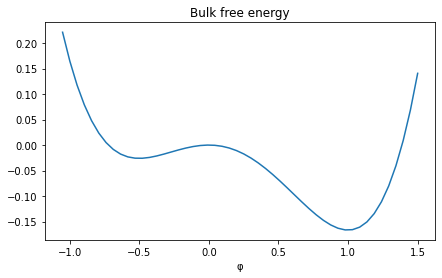
Compared to last tutorial, this bulk free energy has also two minima, but at different values.
Another complexity of the model is its anisotropy. The gradient parameter \(\epsilon\) depends on the interface normal.
[5]:
def σ(θ):
    return 1 + δ * sp.cos(j * (θ - θzero))

θ = sp.atan2(ps.fd.Diff(φ, 1), ps.fd.Diff(φ, 0))

ε_val = εb * σ(θ)
ε_val
[5]:
[6]:
def m_func(T):
    return (α / sp.pi) * sp.atan(γ * (Teq - T))
However, we just insert these parameters into the free energy formulation before doing the functional derivative, to make the dependence of \(\epsilon\) on \(\nabla \phi\) explicit.
[7]:
fe = free_energy_density.subs({
    m: m_func(T),
    ε: εb * σ(θ),
})

dF_dφ = ps.fd.functional_derivative(fe, φ)
dF_dφ = ps.fd.expand_diff_full(dF_dφ, functions=[φ])
dF_dφ
[7]:
Then we insert all the numeric parameters and discretize:
[8]:
discretize = ps.fd.Discretization2ndOrder(dx=0.03, dt=1e-5)
parameters = {
    τ: 0.0003,
    κ: 1.8,
    εb: 0.01,
    δ: 0.02,
    γ: 10,
    j: 6,
    α: 0.9,
    Teq: 1.0,
    θzero: 0.2,
    sp.pi: sp.pi.evalf()
}
parameters
[8]:
[9]:
dφ_dt = - dF_dφ / τ
φ_eqs = ps.simp.sympy_cse_on_assignment_list([ps.Assignment(φ_delta_field.center,
                                                            discretize(dφ_dt.subs(parameters)))])
φ_eqs.append(ps.Assignment(φ_tmp, discretize(ps.fd.transient(φ) - φ_delta_field.center)))

temperature_evolution = -ps.fd.transient(T) + ps.fd.diffusion(T, 1) + κ * φ_delta_field.center
temperature_eqs = [
    ps.Assignment(T, discretize(temperature_evolution.subs(parameters)))
]
When creating the kernels we pass as target (which may be ‘Target.CPU’ or ‘Target.GPU’) the default target of the target handling. This enables to switch to a GPU simulation just by changing the parameter of the data handling.
The rest is similar to the previous tutorial.
[10]:
φ_kernel = ps.create_kernel(φ_eqs, cpu_openmp=4, target=dh.default_target).compile()
temperature_kernel = ps.create_kernel(temperature_eqs, target=dh.default_target).compile()
[11]:
def timeloop(steps=200):
φ_sync = dh.synchronization_function(['phi'])
temperature_sync = dh.synchronization_function(['T'])
dh.all_to_gpu() # this does nothing when running on CPU
for t in range(steps):
φ_sync()
dh.run_kernel(φ_kernel)
dh.swap('phi', 'phi_temp')
temperature_sync()
dh.run_kernel(temperature_kernel)
dh.all_to_cpu()
return dh.gather_array('phi')
def init(nucleus_size=np.sqrt(5)):
for b in dh.iterate():
x, y = b.cell_index_arrays
x, y = x-b.shape[0]//2, y-b.shape[0]//2
bArr = (x**2 + y**2) < nucleus_size**2
b['phi'].fill(0)
b['phi'][(x**2 + y**2) < nucleus_size**2] = 1.0
b['T'].fill(0.0)
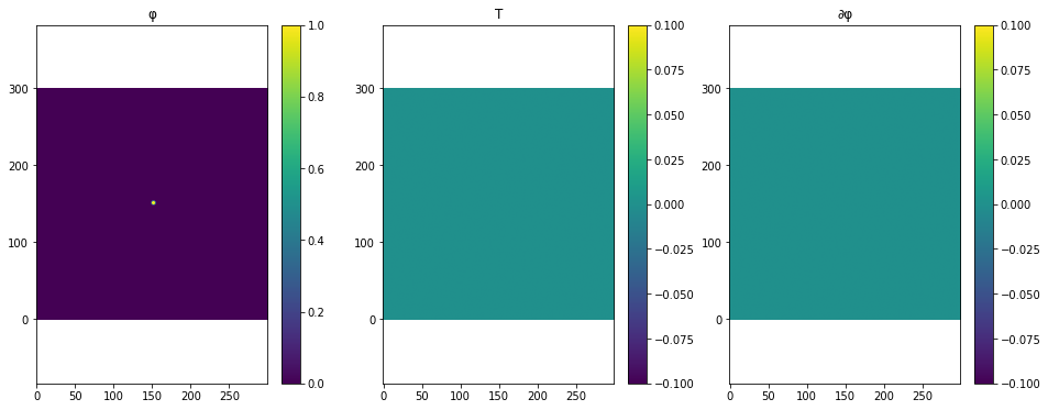
def plot():
plt.subplot(1,3,1)
plt.scalar_field(dh.gather_array('phi'))
plt.title("φ")
plt.colorbar()
plt.subplot(1,3,2)
plt.title("T")
plt.scalar_field(dh.gather_array('T'))
plt.colorbar()
plt.subplot(1,3,3)
plt.title("∂φ")
plt.scalar_field(dh.gather_array('phidelta'))
plt.colorbar()
[12]:
ps.show_code(φ_kernel)
FUNC_PREFIX void kernel(double * RESTRICT const _data_T, double * RESTRICT const _data_phi, double * RESTRICT  _data_phi_temp, double * RESTRICT  _data_phidelta)
{
   #pragma omp parallel num_threads(4)
   {
      #pragma omp for schedule(static)
      for (int64_t ctr_1 = 1; ctr_1 < 301; ctr_1 += 1)
      {
         double * RESTRICT _data_phi_10 = _data_phi + 302*ctr_1;
         double * RESTRICT _data_T_10 = _data_T + 302*ctr_1;
         double * RESTRICT _data_phi_11 = _data_phi + 302*ctr_1 + 302;
         double * RESTRICT _data_phi_1m1 = _data_phi + 302*ctr_1 - 302;
         double * RESTRICT  _data_phidelta_10 = _data_phidelta + 302*ctr_1;
         double * RESTRICT  _data_phi_temp_10 = _data_phi_temp + 302*ctr_1;
         for (int64_t ctr_0 = 1; ctr_0 < 301; ctr_0 += 1)
         {
            const double xi_0 = _data_phi_10[ctr_0]*_data_phi_10[ctr_0];
            const double xi_1 = 954.92965855137209*atan(-10.0 + 10.0*_data_T_10[ctr_0]);
            const double xi_2 = -2222.2222222222222*_data_phi_10[ctr_0];
            const double xi_3 = xi_2 + 1111.1111111111111*_data_phi_11[ctr_0] + 1111.1111111111111*_data_phi_1m1[ctr_0];
            const double xi_4 = cos(-1.2000000000000002 + 6.0*atan2(-16.666666666666668*_data_phi_1m1[ctr_0] + 16.666666666666668*_data_phi_11[ctr_0], -16.666666666666668*_data_phi_10[ctr_0 - 1] + 16.666666666666668*_data_phi_10[ctr_0 + 1]));
            const double xi_5 = xi_4*0.013333333333333336;
            const double xi_6 = xi_2 + 1111.1111111111111*_data_phi_10[ctr_0 + 1] + 1111.1111111111111*_data_phi_10[ctr_0 - 1];
            const double xi_7 = 0.00013333333333333334*(xi_4*xi_4);
            _data_phidelta_10[ctr_0] = xi_0*xi_1 + xi_0*5000.0 + xi_1*-1.0*_data_phi_10[ctr_0] + xi_3*xi_5 + xi_3*xi_7 + xi_5*xi_6 + xi_6*xi_7 - 3148.1481481481483*_data_phi_10[ctr_0] - 3333.3333333333335*(_data_phi_10[ctr_0]*_data_phi_10[ctr_0]*_data_phi_10[ctr_0]) + 370.37037037037038*_data_phi_10[ctr_0 + 1] + 370.37037037037038*_data_phi_10[ctr_0 - 1] + 370.37037037037038*_data_phi_11[ctr_0] + 370.37037037037038*_data_phi_1m1[ctr_0];
            _data_phi_temp_10[ctr_0] = 1.0000000000000001e-5*_data_phidelta_10[ctr_0] + _data_phi_10[ctr_0];
         }
      }
   }
}
[13]:
timeloop(10)
init()
plot()
print(dh)
    Name|      Inner (min/max)|     WithGl (min/max)
----------------------------------------------------
       T|            (  0,  0)|            (  0,  0)
     phi|            (  0,  1)|            (  0,  1)
phi_temp|            (  0,  0)|            (  0,  0)
phidelta|            (  0,  0)|            (  0,  0)
[14]:
result = None
if 'is_test_run' not in globals():
    ani = ps.plot.scalar_field_animation(timeloop, rescale=True, frames=600)
    result = ps.jupyter.display_as_html_video(ani)
result
[14]:
[15]:
assert np.isfinite(dh.max('phi'))
assert np.isfinite(dh.max('T'))