[1]:
from pystencils.session import *
Tutorial 04: Advection Diffusion - Simple finite differences discretization
In this tutorial we demonstrate how to use the discretization layer on top of pystencils, that defines how continuous differential operators are discretized. The result of this discretization layer are stencil equations which are used to generated C or CUDA code.
We are going to discretize the advection diffusion equation without reaction terms:
[2]:
domain_size = (200, 80)
dim = len(domain_size)

# create arrays
c_arr = np.zeros(domain_size)
v_arr = np.zeros(domain_size + (dim,))

# create fields
c, v, c_next = ps.fields("c, v(2), c_next: [2d]", c=c_arr, v=v_arr, c_next=c_arr)

# write down advection diffusion pde
# the equation is represented by a single term and an implicit "=0" is assumed.
adv_diff_pde = ps.fd.transient(c) - ps.fd.diffusion(c, sp.Symbol("D")) + ps.fd.advection(c, v)
adv_diff_pde
[2]:
$\displaystyle \nabla \cdot(v c) - div(D \nabla c) + \partial_t c_{C}$
It describes how the concentration \(c\) of a passive substance, which does not influence the flow field, behaves in a fluid with given velocity \(v\). To illustrate the two effects here, image we release a constant stream of dye at some point in a river. The dye is transported with the flow (advection) but also the trace gets wider and wider normal to the flow direction due to diffusion.
[3]:
discretize = ps.fd.Discretization2ndOrder(1, 0.01)
discretization = discretize(adv_diff_pde)
discretization.subs(sp.Symbol("D"),1)
[3]:
$\displaystyle 0.96 {{c}_{(0,0)}} - 0.005 {{c}_{(1,0)}} {{v}_{(1,0)}^{0}} + 0.01 {{c}_{(1,0)}} - 0.005 {{c}_{(0,1)}} {{v}_{(0,1)}^{1}} + 0.01 {{c}_{(0,1)}} + 0.005 {{c}_{(0,-1)}} {{v}_{(0,-1)}^{1}} + 0.01 {{c}_{(0,-1)}} + 0.005 {{c}_{(-1,0)}} {{v}_{(-1,0)}^{0}} + 0.01 {{c}_{(-1,0)}}$
[4]:
ast = ps.create_kernel([ps.Assignment(c_next.center(), discretization.subs(sp.Symbol("D"), 1))])
kernel = ast.compile()
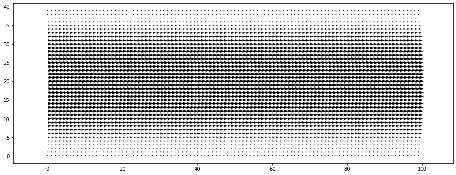
[5]:
y = np.linspace(0, 1, v_arr.shape[1])
v_arr[:, :, 0] = -y * (y - 1.0) * 5
plt.vector_field(v_arr);
[6]:
def boundary_handling(c):
    # No concentration at the upper, lower wall and the left inflow border
    c[:, 0] = 0
    c[:, -1] = 0
    c[0, :] = 0
    # At outflow border: neumann boundaries by copying last valid layer
    c[-1, :] = c[-2, :]

    # Some source inside the domain
    c[10: 15, 25:30] = 1.0
    c[20: 25, 60:65] = 1.0

c_tmp_arr = np.empty_like(c_arr)
def timeloop(steps=100):
    global c_arr, c_tmp_arr
    for i in range(steps):
        boundary_handling(c_arr)
        kernel(c=c_arr, c_next=c_tmp_arr, v=v_arr)
        c_arr, c_tmp_arr = c_tmp_arr, c_arr
    return c_arr
[7]:
if 'is_test_run' in globals():
    timeloop(10)
    result = None
else:
    ani = ps.plot.scalar_field_animation(timeloop, rescale=True, frames=300)
    result = ps.jupyter.display_as_html_video(ani)
result
[7]: